ISO Compliance Insights & Best Practices

Cyber Risk Quantification: A Clear Guide to FAIR Indicators

Cyber risk quantification replaces “high, medium, low” with a number the rest of the business already understands: expected loss in currency, with a range. The dominant method is FAIR — Factor Analysis of Information Risk — which The Open Group publishes as the Open FAIR standard and which decomposes any risk scenario into two measurable branches: how often a loss event happens, and how much it costs when it does. Done properly it produces indicators a board can weigh against a budget; done badly it produces a spreadsheet of invented precision. This guide explains the FAIR model factor by factor, how the indicators it produces differ from a heat map, what data feeds them and where that data comes from, how the results are reported, and the five ways cyber risk quantification programs go wrong.

Cyber risk quantification: the FAIR factors from threat event to loss — Risk decomposes into loss event frequency and loss magnitude; each branch decomposes again into factors that can be estimated with a range.

Why quantify at all

Qualitative risk ratings cannot be added, compared across domains or set against cost. A “high” cyber risk and a “high” supply chain risk say nothing about which deserves the next dollar, and a control that moves a risk from “high” to “medium” cannot be priced. Quantification produces a loss distribution — the probability of losing more than a given amount in a year — and every question a board or a CFO asks follows from it: expected annual loss, the 1-in-10 and 1-in-100 year loss, the reduction a control buys, and therefore its return. It also gives indicators a defined unit, which is what NIST SP 800-55 asks of any measure and what makes cyber risk comparable with the operational and financial risks the enterprise risk function already quantifies.

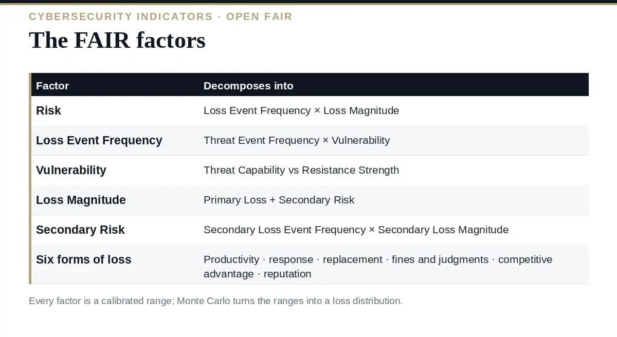
The FAIR model for cyber risk quantification

Open FAIR defines risk as the probable frequency and probable magnitude of future loss, and breaks it into a taxonomy of factors. Each factor is estimated as a range with a most-likely value — a calibrated estimate, not a point — and the ranges are combined by Monte Carlo simulation into a loss distribution.

Factor	Definition	Estimated from
Loss Event Frequency (LEF)	How often, per year, a loss event is expected to occur	Threat Event Frequency × Vulnerability
Threat Event Frequency (TEF)	How often a threat agent acts against the asset in a way that could cause loss	Contact frequency and probability of action; threat intelligence, incident history, industry data
Vulnerability	The probability that a threat event becomes a loss event	Threat Capability vs Resistance Strength — how skilled the attacker is against how strong the control
Loss Magnitude (LM)	The probable loss from a single loss event	Primary Loss + Secondary Risk
Primary Loss	Loss to the primary stakeholder directly from the event	Productivity, response and replacement costs
Secondary Risk	Loss arising from the reactions of secondary stakeholders — customers, regulators, partners	Secondary Loss Event Frequency × Secondary Loss Magnitude: fines and judgments, competitive advantage, reputation

The six forms of loss in Open FAIR — productivity, response, replacement, fines and judgments, competitive advantage, and reputation — are the checklist for loss magnitude. Most organizations can estimate the first three from operations data and the fourth from regulation; the last two are the widest ranges and the ones to show explicitly rather than bury in a mean.

The indicators cyber risk quantification produces

Indicator	What it is	Who uses it
Annualized loss exposure (expected loss)	The mean of the annual loss distribution for a scenario or a portfolio	Budget owners; comparison across risks
Loss at a confidence level	The 90th or 99th percentile annual loss — the 1-in-10 or 1-in-100 year outcome	Boards; risk appetite; insurance limits
Probability of exceeding a threshold	The chance annual loss exceeds a stated amount, e.g. the materiality threshold	Audit committees; disclosure decisions
Control value	The reduction in expected loss or tail loss from a control, against its cost	Investment decisions; the security roadmap
Risk appetite headroom	Distance between current loss exposure and the appetite the board set	Board reporting; the exposure indicator

These are the numbers that belong on the exposure line of board cybersecurity reporting. A heat map cannot produce any of them.

Running a cyber risk quantification

Define the scenario precisely. Asset, threat, effect: “ransomware encrypts the order management system, causing outage”, not “ransomware”. FAIR analyses scenarios; vague scenarios produce vague ranges.
Calibrate the estimators. The ranges are only as good as the people giving them. Calibration training — practising 90% confidence intervals against known answers — is the step most programs skip and the one that separates quantification from guessing.
Estimate each factor as a range. Minimum, most likely, maximum, with the confidence stated. Use data where it exists: incident records for frequency, outage costs for productivity loss, contracts and regulation for fines.
Simulate. Monte Carlo across the ranges, typically tens of thousands of iterations, producing the loss distribution. Open-source and commercial tools exist; a spreadsheet can do it for a handful of scenarios.
Report the distribution, not the mean. Expected loss, the 90th percentile, the probability of exceeding appetite, and the ranges that drove them.
Re-run when something changes. A new control, a new threat report, an incident. The value of quantification is comparison over time and across options.

Where the data comes from

The objection to cyber risk quantification is always data. The answer is that ranges absorb uncertainty — a wide range honestly stated is more useful than a precise category — and that more data exists than most organizations use. Frequency: internal incident and near-miss records, sector ISAC data, breach report series such as the annual Verizon DBIR and Mandiant M-Trends for vector and dwell-time base rates. Vulnerability: control coverage and effectiveness indicators, penetration test results, the CISA Known Exploited Vulnerabilities catalogue for what is actually exploited. Magnitude: business continuity impact analyses for productivity loss, incident retainers and past invoices for response cost, regulatory penalty scales for fines, cyber insurance claims data where the insurer shares it. Our guide to vulnerability management metrics covers the indicators that feed the vulnerability factor.

Five ways cyber risk quantification goes wrong

Point estimates. “Expected loss $2.3m” with no range is a qualitative rating wearing a number. Show the distribution.
Uncalibrated estimators. Ranges given by people who have never been tested are overconfident by habit. Calibrate first.
Scenario sprawl. Fifty scenarios quantified badly are worth less than ten quantified well. Start with the risks the board already worries about.
Quantifying the model, not the business. Loss magnitude has to come from the people who know what an outage costs — operations and finance — not from the security team’s guess.
Reporting once. A single quantification is an anecdote. The indicator is the trend, and the value is in comparing options.

Frequently asked questions

What is cyber risk quantification?
Estimating cyber risk as a probable frequency and probable magnitude of loss, in currency, with ranges — producing indicators such as expected annual loss, loss at a confidence level and control value that can be compared with cost and with other enterprise risks.

What is FAIR?
Factor Analysis of Information Risk, published by The Open Group as the Open FAIR standard. It decomposes risk into loss event frequency and loss magnitude, each broken into estimable factors, combined by Monte Carlo simulation into a loss distribution.

Do we need special software?
Not to start. A calibrated team, a well-defined scenario and a spreadsheet Monte Carlo produce a usable distribution for a few scenarios. Tooling helps when the scenario set grows and results need to be re-run regularly.

How accurate are the numbers?
As accurate as the ranges, which is why the ranges are reported. A wide, honest range is more useful than a precise category; calibration training and real data narrow it over time.

How does this relate to KRIs?
KRIs feed the factors — control coverage and effectiveness indicators inform vulnerability, incident indicators inform frequency — and the quantification’s outputs become the exposure indicators reported to the board.

Where this leaves you

Start cyber risk quantification with the five scenarios the board already asks about, calibrate the people estimating them, estimate every FAIR factor as a range from the best data available, simulate, and report the distribution with its 90th percentile and the headroom against appetite. Then re-run it when a control lands or a threat changes — the indicator is the movement, and it is the one number in security that a CFO will read without translation.

References

The Open Group: Open FAIR — The Open FAIR Risk Taxonomy (O-RT) and Risk Analysis (O-RA) standards.
FAIR Institute — The community and body of knowledge around the FAIR model.
NIST SP 800-55 Vol. 1: Measurement Guide for Information Security — The measure types and documentation fields the quantification indicators should follow.

More on cybersecurity indicators

Cyber risk quantification — you are here
Board cybersecurity reporting: six indicators
The cybersecurity risk register
Cybersecurity KRIs vs KPIs
Vulnerability management metrics
NIST SP 800-55: security measurement

153 key risk and performance indicators keyed to NIST CSF subcategories — the coverage, effectiveness and incident measures that feed the frequency and vulnerability factors — each with a formula, frequency, thresholds and an owner, are in the Excel-based Critical IT and Cybersecurity Indicators templates, or start with the free templates.

Governance Docs

Governance Docs LLC